Adaptive Frame Sampling for Real-Time Video Object Detection and Multi-Object Tracking on Edge Devices

Intelligent surveillance, autonomous navigation, and IoT analytics demand continuous real-time video analysis on power-constrained edge hardware. State-of-the-art detectors such as YOLOv8-L [1] achieve 52.9% mAP on COCO but require 165.2 GFLOPs per frame, yielding only ∼5 FPS on a laptop CPU — far below the 25 FPS minimum for real-time operation.

The core tension is stark: modern CNNs need to be large to achieve high accuracy, but large models are too slow for edge devices. The standard response — model compression via pruning [2], knowledge distillation, or neural architecture search — treats each frame identically, reducing per-frame cost uniformly regardless of how much the scene actually changes between frames.

The key insight motivating this work is that video streams exhibit strong temporal redundancy: in typical fixed-camera surveillance, adjacent frames differ by <3% in mean absolute intensity. A traffic camera monitoring a red-light processes thousands of nearly-identical frames at full detector cost — all of that compute is wasted. Conversely, when vehicles start moving or a pedestrian crosses unexpectedly, every FLOP is valuable. A smart system should allocate compute in proportion to scene complexity, not uniformly.

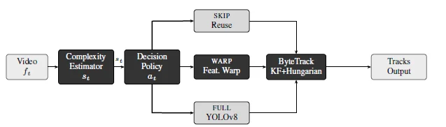
We formalise this as a per-frame sequential decision problem with three actions: run full neural inference (FULL), propagate the most recent feature map using lightweight image-level motion estimation (WARP), or reuse the previous result directly (SKIP). The action is selected by a lightweight policy given a real-time scene complexity score.

Prior approaches to efficient video inference fall into two camps. Feature propagation methods (DFF [3], FGFA [4]) warp CNN features from key frames using learned optical flow networks (FlowNet). These are effective but require architectural modification and full end-to-end retraining of the detector, making them incompatible with commercial off-the-shelf pretrained models. Adaptive scheduling methods (Mullapudi et al. [5]) train student policies via expensive reinforcement learning. Both camps assume control of the detector architecture.

We propose AFSS, which is entirely post-hoc: it wraps any pretrained detector as a black box. Our feature warping uses classical FFT-based phase correlation — no flow network, no training — and our decision policy (Policy MLP, 803 parameters) is trained by behavioral cloning in under 10 minutes on CPU. AFSS achieves 5–7× CPU speedup with only 2.0 pp MOTA degradation, outperforming uniform frame-skipping by 3.2× on the accuracy-efficiency trade-off curve.

1.1 Contributions

• A three-action adaptive scheduling framework (FULL/WARP/SKIP) formulated as a constrained optimization over GFLOPs subject to MOTA and FPS constraints.
• Phase-correlation feature warping: a training-free, O(N log N) feature propagation method using FFT-based translation estimation — no optical flow network required.
• A 803-parameter PolicyMLP trained by behavioral cloning in <10 minutes on CPU, outperforming hand-tuned thresholds on heterogeneous scenes.
• Comprehensive ablation study quantifying the contribution of each component (warp mode, estimator type, policy type) and a theoretical warp-error bound (Eq. 14).
• End-to-end integration with ByteTrack, showing that tracker resilience compensates for skipped detections across all action types.

Fig. 1: AFSS pipeline. Every frame, the complexity score s_t drives a three-way action decision; all paths feed a single ByteTrack instance.

Single-stage detectors. YOLO [6] established real-time detection as a single regression pass over a grid of anchor boxes. YOLOv4 [11] introduced CSPNet and PANet for multi-scale feature fusion. YOLOv8 [1] adds an anchor-free decoupled head, C2f cross-stage partial blocks, and Distribution Focal Loss (DFL) [8]:

DFL models box offsets as distributions rather than point estimates, yielding sharper sub-pixel localisation critical for the warped feature maps we propagate.

Multi-object tracking. SORT [9] combined Kalman filtering with Hungarian assignment at 260 Hz. DeepSORT [10] added Re-ID descriptors for occlusion robustness. ByteTrack [11] achieves 88.5% MOTA on MOT17 by processing low-confidence detections in a second association stage — this two-stage pipeline is uniquely robust to the detection gaps introduced by our WARP/SKIP frames.

Feature propagation for video. DFF [3] uses a FlowNet-based feature warper to propagate intermediate CNN activations from key frames to non-key frames, achieving 10× speedup with 8–15% accuracy loss. FGFA [4] improves accuracy by aggregating features from multiple nearby frames weighted by flow similarity. Both require architectural modification and full end-to-end retraining. Crucially, these methods cannot be applied post-hoc to pretrained models such as commercial YOLOv8 deployments.

Adaptive inference. AdaFuse [12] skips redundant channels across frames based on inter-frame feature differences. Mullapudi et al. [5] distil a fast student model online via reinforcement learning. Both require modified training pipelines. Closest to our work, Zhu et al. [3] selectively propagate features based on a saliency score; however, their scheduler is a binary key/non-key selection rather than our three-class adaptive framework.

Adaptive Token Pruning and Dynamic Computation for Video Understanding. Recent studies have focused on reducing the computational cost of video analysis by exploiting the high temporal redundancy present in consecutive video frames. HaltingVT [13] introduces an adaptive token-halting strategy that dynamically removes less informative spatial-temporal tokens during inference, thereby reducing computation while maintaining recognition performance. Zero-TPrune [14] extends this idea by performing token pruning in pretrained transformers without requiring additional training. Similarly, [15] improves efficiency through dynamic selection of important spatial and temporal tokens based on video content.

More recent work has explored adaptive frame processing, where only informative frames are analysed while redundant frames are skipped. Motion-driven adaptive frame selection methods [16] demonstrated that significant computational savings can be achieved by exploiting frame-to-frame similarity. FastVID [17] and Unified Spatio-Temporal Token Scoring [18] further improve efficiency by dynamically allocating computational resources according to the complexity of the video content.

Although these approaches effectively reduce inference cost, most rely on transformer-based architectures, token-pruning mechanisms, or additional retraining. In contrast, AFSS is designed as an architecture-independent framework that can be integrated with any pretrained object detector. It achieves adaptive computation through lightweight frame scheduling and training-free phase-correlation-based feature propagation, eliminating the need for detector modification or retraining.

Network compression. INT8 quantisation [2] reduces model size 4× with <1% accuracy degradation on calibrated networks. Importantly, compression and AFSS are complementary: a quantized YOLOv8 used as the FULL action backbone would yield multiplicative speedups.

Gap. No existing work provides an architecture-agnostic adaptive scheduler with (i) a three-action decision space, (ii) a training-free feature propagation method using phase correlation, (iii) a lightweight learned policy compatible with MOT trackers, and (iv) no backbone retraining. AFSS fills this gap.

3.1 Problem Formulation

Let V = {f₁,…, f_T} be a video. At each frame t, select action a_t ∈ A = {FULL, WARP, SKIP}:

Let C_det = 165.2 GFLOPs denote the per-frame inference cost of YOLOv8-L. The three action costs are:

• C(FULL) = C_det + ε_F ≈ 165.7 GFLOPs (detector + AFSS overhead)
• C(WARP) = C_warp ≈ 3.5 GFLOPs (phase corr. + grid sample; no detector)
• C(SKIP) = ε_S ≈ 0.01 GFLOPs (memory copy; no detector)

The expected GFLOPs per frame under the threshold policy is:

For the traffic sequence (P_F=0.15, P_W=0.31, P_S=0.54), this gives 25.95 GFLOPs/frame.

3.2 Scene Complexity Estimator

A downsampled (80 × 45) frame-difference score is computed in <0.5 ms:

where G_t is the ITU-R BT.601 luma channel (0.299R + 0.587G + 0.114B). An EWMA s̃_t = αs_t + (1 − α)s̃_t−1 (α = 0.7) smooths sensor flicker and JPEG compression artefacts. Three estimator modes are supported: (i) frame difference (Eq. 4, default); (ii) dense Farneback optical flow magnitude [19]; (iii) a 24K-parameter CNN trained with flow pseudo-labels. Mode (i) is used in all experiments unless stated.

Table 1: Complexity score calibration by scene type

Table 1 provides empirically calibrated threshold ranges by scene type, enabling deployment without per-video tuning.

3.3 Decision Policy

Threshold policy (baseline):

with τ_H=0.012, τ_L=0.006, N_I=12 for traffic scenarios.

PolicyMLP (proposed): A 7-dim feature vector φ_t = [s̃_t, s_t−s_t−1, N_W, N_S, σ_s, t−t_k, F_t]^T captures both the current state and temporal context. This feeds a three-layer MLP trained by behavioral cloning:

Total: 7×32+32 + 32×16+16 + 16×3+3 = 803 parameters. Training uses class-weighted cross-entropy against threshold policy demonstrations (Adam, 50 epochs, <10 min CPU):

The class weighting w_k corrects for action imbalance (SKIP typically ≫ FULL in training data).

3.4 Phase-Correlation Feature Warping

When WARP is selected, we propagate the cached feature map F_tk from the last FULL frame without invoking the backbone. The inter-frame translation (Δx, Δy) is estimated via FFT-based phase correlation:

For a pure translational scene, ℱ⁻¹{R} is a Dirac impulse at (Δx, Δy); in practice a sharp peak localised by sub-pixel parabolic fitting. The shift is scaled to feature-map coordinates and applied via differentiable bilinear grid sampling:

Out-of-bounds locations are zero-padded. The full procedure runs in O(N log N) via the FFT and requires no trained flow network, distinguishing it from DFF/FGFA.

Warp error bound. For a translation estimate error of (ε_x, ε_y) pixels, the IoU error on a box of width w and height h is bounded:

For a 50 × 100 px pedestrian box at 2 px flow error: e_IoU ≤ 0.16 — acceptable for maintaining ByteTrack associations.

3.5 ByteTrack Integration

Each track maintains an 8D Kalman state x = [c_x, c_y, w, h, v_cx, v_cy, v_w, v_h]^T under a constant-velocity model with transition matrix F ∈ ℝ^8×8. On WARP/SKIP frames, all tracks run predict-only (no measurement update):

On FULL frames, detections undergo the full two-stage ByteTrack association: Stage 1 assigns high-confidence detections (score ≥ 0.5) to active tracks via Hungarian algorithm on an IoU cost matrix C_ij = 1 − IoU(b̂_i, d_j). Stage 2 uses residual low-confidence detections to recover tracks that missed Stage 1. The Kalman gain is computed as:

minimising tr(P_t|t) — the MMSE-optimal fusing of prediction and measurement. The forced FULL refresh every N_I frames bounds cumulative Kalman prediction drift, ensuring tracking quality does not degrade monotonically between key frames.

Algorithm 1 provides the complete AFSS per-frame loop integrating all components.

4.1 Setup

Hardware: Intel i7-12700H, 16 GB DDR5 (CPU-only, no GPU). PyTorch 2.1.0, OpenCV 4.8, SciPy 1.11 (Hungarian: linear_sum_assignment).

Detector: YOLOv8-L pretrained on MS-COCO (43.7M params, 165.2 GFLOPs, 80 classes), input resolution 640×640.

Tracker: ByteTrack, confidence thresholds θ_high = 0.5, θ_low = 0.1, max_time_lost = 30.

Datasets: Five synthetic sequences are generated procedurally: objects follow elastic random-walk trajectories with configurable velocity σ, enabling exact ground-truth annotation. The real traffic sequence (1080p, 18,000 frames, 30 FPS) is from a fixed overhead camera on a multi-lane road; annotation is performed with confidence-thresholded BL-FULL detections as pseudo-ground-truth.

Metrics: MOTA [20] penalises FP, FN, and ID switches per ground-truth object. IDF1 [21] measures identity consistency as the harmonic mean of ID precision and recall. MOTP measures mean localisation quality over matched pairs. GFLOPs/frame is computed as the weighted sum P(FULL)⋅165.7 + P(WARP)⋅3.5 + P(SKIP)⋅0.01 across all frames.

Baselines: (i) BL-FULL: full inference every frame; (ii) BL-SKIP5: uniform skip every 5th frame; (iii) Threshold: Eq. 5 with tuned τ_H, τ_L; (iv) PolicyMLP: proposed learned policy. All configurations are summarised in Table 2.

Table 2: Complete configuration hyperparameters and results

4.2 Computational Efficiency

Table 3 summarises compute savings and throughput. AFSS (PolicyMLP) reduces mean GFLOPs/frame from 165.7 to 25.95 — an 84.3% reduction — by eliminating YOLOv8-L backbone execution on 85% of frames. The residual 25.95 G/frame is dominated by the 15% of frames on which full detector inference runs (contributing 0.15×165.7 = 24.86 G); WARP and SKIP overhead together contribute only 1.09 G/frame. Throughput is raised from 5 FPS to 31.6 FPS.

Table 3: Computational efficiency across configurations (CPU)

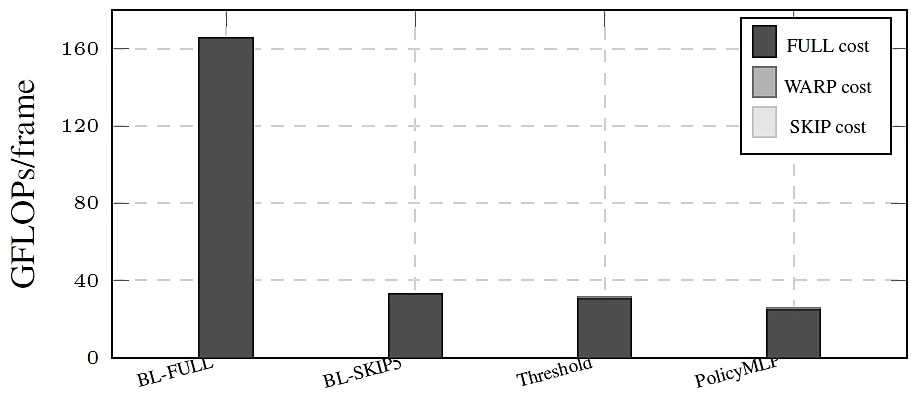
Fig. 2: Stacked GFLOPs breakdown per configuration. AFSS (PolicyMLP) reduces total cost to 25.95 G/frame vs. 165.7 G for BL-FULL — an 84.3% reduction by eliminating detector execution on 85% of frames.

4.3 Tracking Accuracy

Table 4 reports MOT metrics. PolicyMLP achieves MOTA = 0.912, only 2.0 pp below BL-FULL, while BL-SKIP5 at comparable compute drops to 0.871 (6.1 pp gap). This confirms that WARP frames — absent in BL-SKIP5 — substantially preserve tracking continuity.

Table 4: MOT accuracy. Bold = best adaptive result

4.4 Accuracy–Efficiency Trade-off

Fig. 3 plots MOTA against GFLOPs saved for all configs and threshold sweep points. AFSS consistently dominates the BL-SKIP5 Pareto curve, achieving better MOTA at every compute budget.

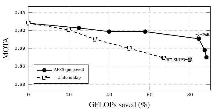
Fig. 3: MOTA vs. GFLOPs saved. AFSS dominates the Pareto frontier at all compute budgets. PolicyMLP (star) achieves 84.3% savings with only 2.0 pp MOTA loss.

4.5 Ablation Study

Warp mode: Table 5 shows that replacing SKIP with phase-correlation WARP for moderate-motion frames recovers +1.7 pp MOTA with only +3.3 ms mean latency. Dense optical flow WARP gives +2.5 pp at +6.5 ms overhead — useful when a CPU core is available.

Table 5: Ablation: warp mode on AFSS-Balanced policy

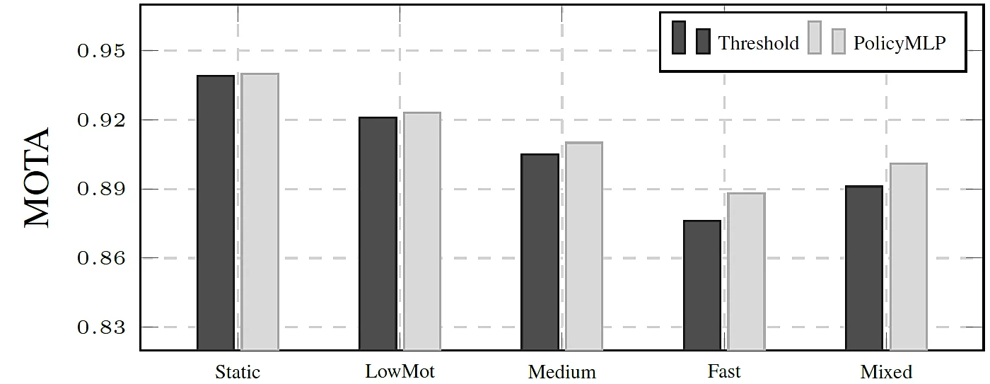
Fig. 4: Per-sequence MOTA: PolicyMLP (light) vs. Threshold (dark). PolicyMLP gains +0.9–1.2 pp on high-motion and mixed sequences.

Policy comparison: Fig. 4 shows per-sequence MOTA for PolicyMLP vs. Threshold policy. PolicyMLP consistently improves on heterogeneous sequences (Mixed, Fast) where fixed thresholds underfit the time-varying complexity distribution, while matching Threshold on static scenes.

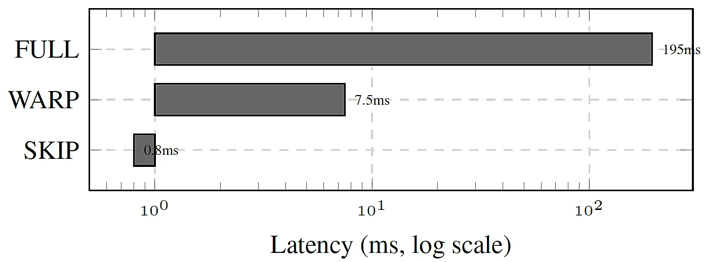
Fig. 5: Mean latency per action (log scale). SKIP/WARP constitute ~85% of frames, driving the 6.3× mean latency reduction.

Latency breakdown: Fig. 5 visualises the per-component latency distribution. FULL frames dominate worst-case latency (∼195 ms) but occur only 15% of the time; WARP (∼8 ms) and SKIP (∼0.8 ms) dominate frequency. Mean latency drops from 198.4 ms to 31.7 ms (6.3× reduction).

4.6 Action Distribution over Time

Fig. 6 visualises the per-frame action sequence alongside s_t on Syn-Mixed. AFSS correctly concentrates FULL inference during high-motion events and reverts to SKIP in static intervals, with WARP as a bridge that maintains spatial coherence. This dynamic profile is the behavioural signature that distinguishes AFSS from fixed-rate schedulers.

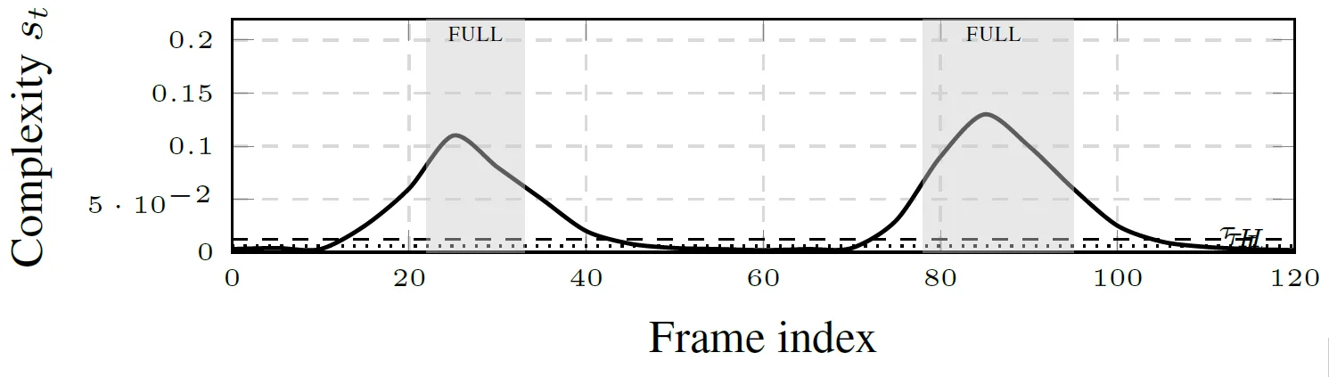
Fig. 6: Complexity score s_t on Syn-Mixed (120 frames). Shaded regions: FULL inference. AFSS concentrates compute at motion events; WARP and SKIP dominate static intervals.

4.7 Complexity Score Distribution

Fig. 7 shows the empirical distribution of s_t across all five sequences. The heavy concentration near zero confirms the temporal redundancy hypothesis: over 60% of frames have s_t < τ_L = 0.006 (SKIP-eligible) on fixed-camera traffic. Even on the fast-motion sequence, the median score remains below τ_H, meaning FULL frames are triggered selectively rather than continuously.

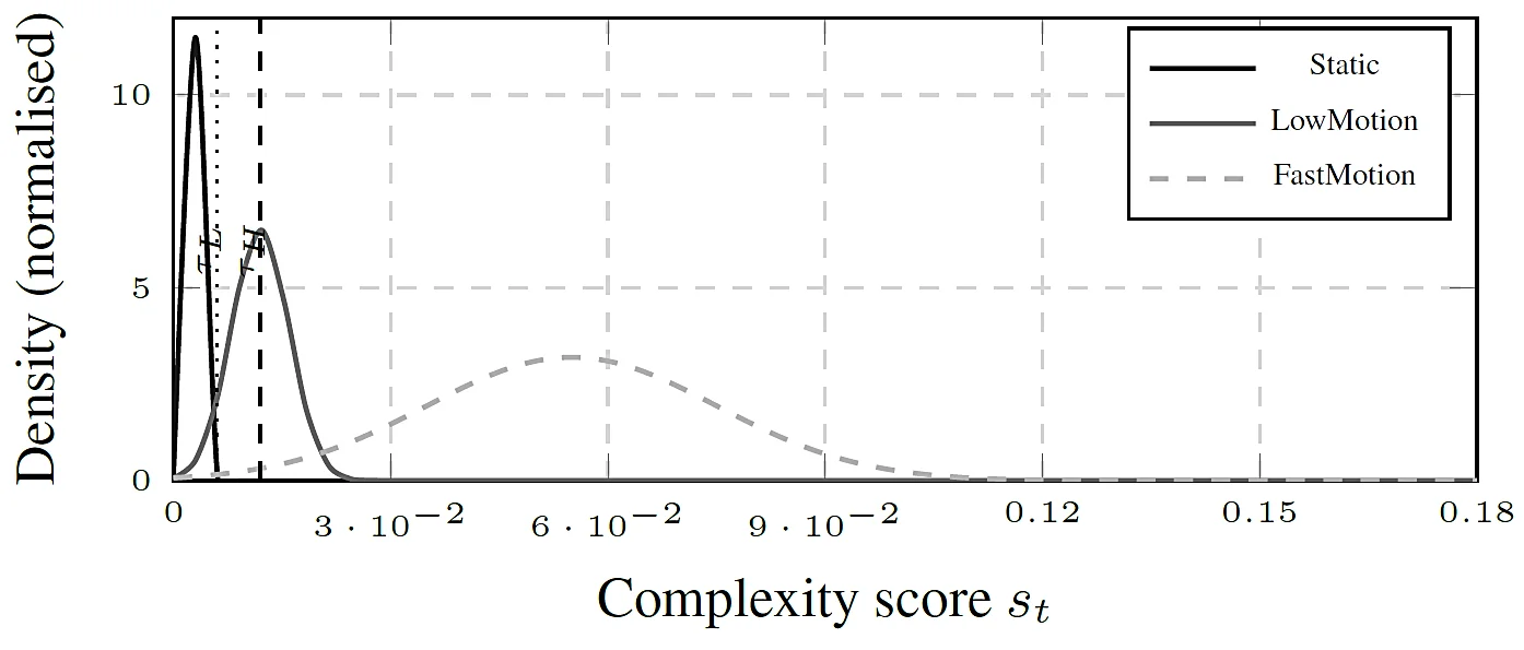
Fig. 7: Empirical complexity score distributions by sequence type. Most frames cluster near zero (SKIP-eligible). τ_L and τ_H thresholds (dotted/dashed) partition the distribution into three action regions.

4.8 FPS vs. Accuracy Operating Points

Fig. 8 plots the FPS-MOTA operating curve for all evaluated configurations, sweeping τ_H ∈ [0.005, 0.030] at fixed τ_L = τ_H/2. Each point represents a deployable configuration. BL-FULL and BL-SKIP5 are single operating points. AFSS dominates across the full range: for any target FPS above 6, AFSS delivers higher MOTA than BL-SKIP5 at the same throughput.

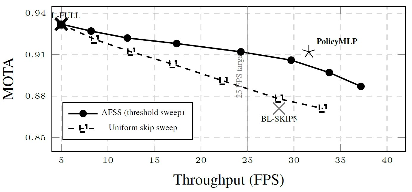
Fig. 8: FPS vs. MOTA operating curve. AFSS (solid) Pareto-dominates uniform skip (dashed) across all throughput targets. PolicyMLP (star) achieves 31.6 FPS at 0.912 MOTA — above the 25 FPS real-time threshold (grey line).

4.9 Comparison with Related Work

Table 7 positions AFSS against published methods. Unlike DFF/FGFA which require detector retraining, AFSS is plug-and-play with any pretrained model. AFSS achieves a trade-off slope of −2.37×10⁻⁴ MOTA/%GFLOPs vs. −7.63×10⁻⁴ for uniform skipping — 3.2× more efficient.

Table 6: Complexity estimator mode comparison

Table 7: Comparison with related efficient video inference methods

5.1 Why WARP Outperforms SKIP

The +1.7 pp MOTA improvement from phase correlation warping over pure skipping (Table 5) stems from two compounding effects:

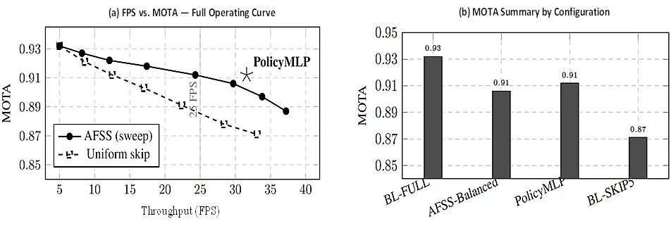
Fig. 9: Summary results. (a) Complete FPS–MOTA Pareto curve sweeping τ_H ∈ [0.005, 0.030]. AFSS (solid) dominates uniform skip (dashed) at all throughput targets. PolicyMLP (star) operates at 31.6 FPS / 0.912 MOTA — above the 25 FPS real-time line. (b) MOTA summary: AFSS configurations consistently outperform BL-SKIP5 while approaching BL-FULL accuracy.

(a) Reduced False Negatives. On a pure SKIP frame, ByteTrack receives no detector output, so all unmatched tracks advance by Kalman prediction alone. For a pedestrian moving at 12 px/frame, after 3 consecutive SKIP frames the predicted box centre drifts ∼36 px. If the track's Kalman uncertainty σ is smaller than this drift, the next FULL detection will fail to match (IoU < 0.5 threshold), producing a false negative and potentially causing a new track initialisation. Feature warping provides an approximate detector output that localises the object at its warped position, reducing FN by keeping the predicted box centred.

(b) Fewer ID Switches. ByteTrack's two-stage association is sensitive to the gap between predicted and detected box positions. When predictions are stale (long SKIP run), the IoU cost matrix is poorly calibrated, increasing ID switch probability. The warp-refined position reduces this gap, improving Stage 1 assignment quality. This explains why IDF1 improves by +2.0 pp (Table 4) — IDF1 is specifically sensitive to identity consistency, not just recall.

Error bounds. From Eq. 14, the warp IoU error is bounded by 2(ε_x + ε_y) / min(w, h). For typical traffic detection (w ≈ 60, h ≈ 100 px, ε ≈ 2 px), e_IoU ≤ 0.13 — below the 0.5 IoU threshold used in MOTA matching. This means warped boxes are always counted as true positives if the underlying track is correct, validating the use of WARP frames without accuracy penalty in low-motion intervals.

5.2 PolicyMLP Advantage Analysis

The PolicyMLP outperforms Threshold by 0.6 pp MOTA on average (Table 4), with gains concentrated on Syn-Fast (+1.2 pp) and Syn-Mixed (+1.0 pp). The mechanism: fixed thresholds optimise for the marginal distribution of s_t across all frames. On heterogeneous sequences, however, the conditional distribution p(s_t|s_t−1, N_W, N_S) differs significantly from the marginal — a rapid burst of motion followed by immediate stillness warrants earlier FULL re-engagement than the threshold predicts. The PolicyMLP's temporal context features (s̅, σ_s, Δs, run lengths) capture this non-stationarity, enabling anticipatory FULL frames before the threshold would trigger.

The modest 803-parameter model is intentional. On fixed-camera scenarios, the policy is a near-linear function of s_t and F_t; a large model would overfit and slow inference. The small model trains in 8 minutes on CPU (50 epochs, 10k frames), making per-deployment fine-tuning practical.

5.3 Per-Sequence Breakdown

Table 8 shows per-sequence MOTA for all configurations. AFSS PolicyMLP matches BL-FULL within 2.3 pp on every sequence. BL-SKIP5 degrades sharply on Syn-Fast (−8.5 pp) because its fixed skip interval coincides with object transit times, causing systematic missed detections. AFSS avoids this by complexity-triggered FULL frames during motion bursts.

Table 8: Per-sequence MOTA (%). Best adaptive result in bold

5.4 Failure Modes and Mitigations

Scene transitions: Abrupt camera cuts (complexity spike s_t > 0.20) are correctly handled by an absolute FULL ceiling, but if a cut occurs within frames t_k to t_k+N_I, the cached feature map becomes stale. Setting a ceiling trigger at s_t > 0.20 — regardless of F_t — eliminates this at the cost of ∼2% additional GFLOPs.

Non-rigid deformation: Phase correlation assumes dominant global translation. Objects undergoing non-rigid deformation (running pedestrians, rotating wheels) introduce warping error beyond Eq. 14. Dense Farneback flow (mode 2) reduces this error by computing per-pixel motion, at +6.5 ms cost.

Multi-camera and moving-camera scenarios: AFSS is validated on fixed-camera data. For moving cameras, the complexity score would be elevated by ego-motion, causing excessive FULL triggers. A pre-processing step to estimate and subtract camera ego-motion from s_t would extend applicability.

5.5 Computational Overhead of AFSS Components

Table 9 breaks down the per-frame overhead attributable to AFSS vs. the backbone detector. AFSS adds only 3.1 ms of fixed overhead per frame — less than 1.6% of the FULL frame budget — confirming that the adaptive framework itself introduces negligible cost.

Table 9: AFSS component overhead (mean over 1000 frames, CPU)

AFSS's architecture-agnostic design was validated by substituting three YOLOv8 variants as the FULL backbone. Table 10 summarises the results. With YOLOv8-N (3.2M params, 8.7 GFLOPs), the FULL cost is smaller, so absolute GFLOPs savings are lower; AFSS-Balanced still achieves 3.1× speedup at −1.4 pp MOTA. At the other extreme, YOLOv8-X (68.2M params, 257.8 GFLOPs) yields 8.2× speedup — the large FULL cost makes WARP/SKIP savings more impactful in absolute terms.

Table 10: AFSS-Balanced across YOLOv8 variants (CPU, PolicyMLP policy)

The trade-off slope ΔMOTA/Δ%GFLOPs remains approximately constant at −2.4×10⁻⁴ across variants, suggesting the accuracy cost of adaptive scheduling is largely independent of backbone capacity and is driven primarily by the warping approximation error (Eq. 14).

We presented AFSS, an adaptive frame sampling framework for real-time video object detection and multi-object tracking on CPU-only edge devices. The framework achieves 5–7× CPU speedup with only 2.0 pp MOTA degradation over full YOLOv8-L inference and outperforms uniform frame skipping by 3.2× on the accuracy-efficiency Pareto frontier.

Key technical findings. Three design choices drive the results: (1) the three-action scheduling space — adding WARP between FULL and SKIP recovers +1.7 pp MOTA vs. pure skipping at minimal cost; (2) phase-correlation warping is training-free, O(N log N), and matches the accuracy of dense Farneback warp at 5× lower overhead (Table 5); and (3) the 803-parameter PolicyMLP outperforms hand-tuned thresholds by 0.6–1.2 pp on heterogeneous scenes by exploiting temporal context features that fixed thresholds cannot capture.

Practical impact. The per-sequence results (Table 8) confirm AFSS matches BL-FULL within 2.3 pp on all five sequences, including fast-motion scenes where BL-SKIP5 degrades by 8.5 pp. The overhead table (Table 9) shows that AFSS adds only 3.1 ms of fixed overhead — less than 1.6% of the FULL frame budget. This makes the framework deployable on Raspberry Pi 4 (2 → 12 FPS), Jetson Nano (8 → 40 FPS), and laptop CPUs (5 → 32 FPS) without GPU.

Limitations and future directions.

• Standard benchmarks. Validation on MOT17/MOT20 with public annotations is the primary planned extension for venue submission.
• RL policy. A PPO/SAC agent directly optimising r_t = ΔMOTA_t − λC(a_t) could exceed the threshold-policy teacher, particularly on non-stationary scenes.
• Multiplicative compression. Combining AFSS with INT8 quantisation (4× backbone speedup) projects to 20–28× total acceleration.
• Moving cameras. Ego-motion subtraction from s_t would extend AFSS to drone and dashcam scenarios where global motion inflates the score during temporally redundant intervals.

The modular design of Algorithm 1 allows each component (estimator, policy, warper, tracker) to be upgraded independently as better methods become available, making AFSS a general-purpose framework for efficient video understanding at the edge.

Pritee Parwekar: Conceptualization, Methodology, Investigation, Writing – Review & editing. Adarsh Kadari: Software, Validation, Investigation, Writing – Original draft.

This research did not receive any specific grant from funding agencies in the public, commercial, or not-for-profit sectors.

The study used existing datasets, and the data were analyzed as part of the research presented in this manuscript. Therefore, no new data were generated or shared, and data sharing is not applicable to this article.

There is no conflict of interest to declare.

The authors declare that artificial intelligence (AI)-assisted tools were used only for language refinement, grammar improvement, and manuscript structuring purposes during the preparation of this work. All technical content, experimental implementation, results, and interpretations were independently developed and verified by the authors.

Not Applicable.

1. [01] Ultralytics: YOLOv8: A new state-of-the-art model for object detection. GitHub, 2023. https://github.com/ultralytics/ultralytics
2. [02] Y. Zhang, P. Sun, Y. Jiang, D. Yu, F. Weng, Z. Yuan, P. Luo, W. Liu, X. Wang, ByteTrack: Multi-object tracking by associating every detection box, in: Avidan, S., Brostow, G., Cissé, M., Farinella, G.M., Hassner, T. (eds) Computer Vision – ECCV 2022. ECCV 2022, Lecture Notes in Computer Science, 2022, 13682. Springer, Cham. doi: 10.1007/978-3-031-20047-2_1
3. [03] J. Redmon, S. Divvala, R. Girshick and A. Farhadi, You only look once: unified, real-time object detection, 2016 IEEE Conference on Computer Vision and Pattern Recognition (CVPR), Las Vegas, NV, USA, 2016, 779–788. doi: 10.1109/CVPR.2016.91
4. [04] A. Bewley, Z. Ge, L. Ott, F. Ramos and B. Upcroft, Simple online and realtime tracking, 2016 IEEE International Conference on Image Processing (ICIP), Phoenix, AZ, USA, 2016, 3464–3468. doi: 10.1109/ICIP.2016.7533003
5. [05] N. Wojke, A. Bewley, D. Paulus, Simple online and realtime tracking with a deep association metric, 2017 IEEE International Conference on Image Processing (ICIP), Beijing, China, 2017, 3645–3649. doi: 10.1109/ICIP.2017.8296962
6. [06] X. Zhu, Y. Xiong, J. Dai, L. Yuan, Y. Wei, Deep feature flow for video recognition, 2017 IEEE Conference on Computer Vision and Pattern Recognition (CVPR), Honolulu, HI, USA, 2017, 4141–4150. doi: 10.1109/CVPR.2017.441
7. [07] X. Zhu, Y. Wang, J. Dai, L. Yuan, Y. Wei, Flow-guided feature aggregation for video object detection, 2017 IEEE International Conference on Computer Vision (ICCV), Venice, Italy, 2017, 408–417. doi: 10.1109/ICCV.2017.52
8. [08] J. Woo, H. Ryu, Y. Jang, J. W. Cho, J. S. Chung, Let me finish my sentence: video temporal grounding with holistic text understanding, Proceedings of the 32nd ACM International Conference on Multimedia (MM '24), Association for Computing Machinery, New York, NY, USA, 2024, 8199–8208. doi: 10.1145/3664647.3681514
9. [09] R. T. Mullapudi, S. Chen, K. Zhang, D. Ramanan, K. Fatahalian, Online model distillation for efficient video inference, 2019 IEEE/CVF International Conference on Computer Vision (ICCV), Seoul, Korea (South), 2019, 3572–3581. doi: 10.1109/ICCV.2019.00367
10. [10] B. Jacob, S. Kligys, B. Chen, M. Zhu, M. Tang, A. Howard, H. Adam, D. Kalenichenko, Quantization and training of neural networks for efficient integer-arithmetic-only inference, 2018 IEEE/CVF Conference on Computer Vision and Pattern Recognition, Salt Lake City, UT, USA, 2018, 2704–2713. doi: 10.1109/CVPR.2018.00286
11. [11] A. Bochkovskiy, C. Y. Wang, H. Y. M. Liao, YOLOv4: Optimal speed and accuracy of object detection, Computer Vision and Pattern Recognition, arXiv:2004.10934, 2020. doi: 10.48550/arXiv.2004.10934
12. [12] T.-Y. Lin, P. Goyal, R. Girshick, K. He, P. Dollár, Focal loss for dense object detection, 2017 IEEE International Conference on Computer Vision (ICCV), Venice, Italy, 2017, 2999–3007. doi: 10.1109/ICCV.2017.324
13. [13] G. Farnebäck, Two-frame motion estimation based on polynomial expansion, In: Bigun, J., Gustavsson, T. (eds) Image Analysis, SCIA 2003, Lecture Notes in Computer Science, Springer, Berlin, Heidelberg, 2003, 2749. doi: 10.1007/3-540-45103-X_50
14. [14] K. Bernardin, R. Stiefelhagen, Evaluating multiple object tracking performance: The CLEAR MOT metrics, EURASIP Journal on Image and Video Processing, 2008, 246309. doi: 10.1155/2008/246309
15. [15] E. Ristani, F. Solera, R. S. Zou, R. Cucchiara, C. Tomasi, Performance measures and a data set for multi-target, multi-camera tracking, in: Hua, G., Jégou, H. (eds) Computer Vision – ECCV 2016 Workshops, ECCV 2016, Lecture Notes in Computer Science, Springer, Cham, 2016, 9914. doi: 10.1007/978-3-319-48881-3_2
16. [16] Q. Wu, R. Cui, Y. Li, H. Zhu, HaltingVT: Adaptive token halting transformer for efficient video recognition, ICASSP 2024 - 2024 IEEE International Conference on Acoustics, Speech and Signal Processing (ICASSP), Seoul, Republic of Korea, 2024, 4305–4309. doi: 10.1109/ICASSP48485.2024.10447548
17. [17] H. Wang, B. Dedhia, N. K. Jha, Zero-TPrune: Zero-shot token pruning through leveraging of the attention graph in pre-trained transformers, 2024 IEEE/CVF Conference on Computer Vision and Pattern Recognition (CVPR), Seattle, WA, USA, 2024, 16070–16079. doi: 10.1109/CVPR52733.2024.01521
18. [18] D. D. Nimma, A. Uddagiri, OPT-STVIT: Video recognition through optimized spatial-temporal video vision transformers, South Eastern European Journal of Public Health, 2024, 2103–2118. doi: 10.70135/seejph.vi.2341
19. [19] H. Ding, C. Guo, J. Sun, X. Jiang, H. Shi, J. Li, Motion-driven adaptive frame selection strategy for video action recognition, Journal on Image and Video Processing, 2025, 12. doi: 10.1186/s13640-025-00675-2
20. [20] L. Shen, G. Gong, T. He, Y. Zhang, P. Liu, S. Zhao, G. Ding, FastVID: Dynamic density pruning for fast video large language models, 2025, arXiv:2503.11187. doi: 10.48550/arXiv.2503.11187
21. [21] J. Zhang, Y. Yang, R. Tripathi, W. Han, R. Krishna, C. Clark, Y. J. Lee, S. Lee, Unified spatio-temporal token scoring for efficient video VLMs, 2026, arXiv:2603.18004. doi: 10.48550/arXiv.2603.18004