

 Open Access||Research Article
Smart Farming and Crop Protection by Evaluating the Performance of Convolutional Neural Networks and YOLOv4 for Plant Leaf Disease Detection
Department of Electronics and Telecommunications Engineering, Sinhgad Institute of Technology, Lonavala, Maharashtra, 410401, India
Abstract
Agriculture plays a significant role in India due to population growth and increased food demands. Hence, there is a need to enhance the yield of crops. Vegetation is frequently susceptible to a wide range of diseases that arise due to various seasonal and environmental conditions. These plant diseases not only jeopardize the quality and quantity of agricultural produce but also pose serious threats to farmers' livelihoods and overall food security. Traditionally, the identity and treatment of plant diseases have relied closely on guide inspection and professional understanding, which may be time-consuming and susceptible to human mistakes. With recent advancements in technology, there is a growing interest in automated disease detection systems that leverage artificial intelligence and machine learning techniques. These contemporary solutions provide faster, more accurate and cost-effective techniques for identifying plant diseases, permitting farmers to take properly timed preventive and corrective measures. This study presents a novel approach to plant leaf disease detection and severity classification by leveraging the capabilities of YOLOv4 and Convolutional Neural Networks (CNNs). These machine learning algorithms have proven great potential in image processing and pattern recognition tasks, making them appropriate for diagnosing plant situations from visual information. We have used a dataset containing images of four various plant species, each suffering from different kinds of infections. By training these models by available datasets, the proposed system can recognize and classify diverse plant diseases with high accuracy. The performance parameters are evaluated extensively and results are derived. The accuracy of the CNN and YOLOv4 obtained around 95.5% & 91.0%, respectively.
Keywords
Graphical Abstract
Novelty Statement
A novel approach to plant disease detection and severity classification by leveraging the capabilities of YOLOv4 and Convolutional Neural Networks (CNNs).
1. Introduction
Agriculture plays a vital role in the Indian economy providing food security for its large population, employing a significant portion of the workforce, contributing to the country's Gross Domestic Product (GDP). Therefore, maintaining the quality, quantity, and health of crops is essential. Due to the unexpected rise in food consumption caused by a population explosion, plant diseases have become a major concern in every country.[1]
Based on the latest projections from the United Nations Food and Agriculture Organization (FAO), plant diseases cause over 40% of the world's vegetation to die every year. Numerous seasonal variables, animate (weeds and pests), and inanimate (weather, rainfall, wind, and moisture) factors can all cause different types of diseases to infect the plants. Plant disease detection can aid farmers in diagnosing and treating comparable conditions, which will improve food safety and profitability. One of the factors affecting the quality and quantity of agricultural production is the influence of plant disease.[2]
Recent trends present new opportunities for agricultural imaging. It is possible to identify folate diseases and show the health of plants by examining the visually noticeable patterns of plant leaves. As a result, it provides a means to significantly decrease yield loss and boost plant production.[3] Many machine learning methods have been employed extensively to detect various plant diseases based on infected leaves. To improve accuracy, this research employs deep learning models such as Dense Net and Efficient Net to detect plant diseases and identify their severity, using a support vector machine. Farmers implement significant mitigations as soon as possible since they are aware of how serious the disease is.[3]
Most of the literature on plant diseases looks at them from a biological standpoint. Their predictions are based on the exposed leaf and plant surfaces. Finding the first signs of disease is one of the most crucial steps in properly managing it. Human experts have historically detected. Blind diseases can be identified by human doctors, despite some obstacles that may hinder their efforts. In this setting, plant disease prevalence has a detrimental effect on agricultural productivity if infections are not identified quickly.[4] It is crucial for managing agricultural output and decision-making.
Plant disease identification has grown to be a significant challenge in recent years. Infected plants typically exhibit visible flaws or lesions in their leaves, branches, blooms, or fruits. Variations in each disease or pest state can typically be recognized by their distinct visual patterns. Plant leaves are the primary source of information on plant diseases because most disease symptoms may initially manifest on the leaf.[5]
3. Dataset
Images of plant leaves from Plant Village were used to see the overall performance. A total of 65,345 plant leaves, including both healthy and diseased samples, were collected and are known as the Plant Village Dataset (Plant Village).
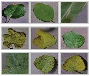
Apple, blue berry, etc. are among the fourteen amazing crop varieties that are included in the databases. A selection of example photos is shown in Fig. 1, which displays the number of image files collected for lesion diagnosis and detection. The availability of water, vitamins, microorganisms, viruses, and fungus are examples of common stressors that lead to sickness.[12]
Fig. 1 shows sample examples of plant leaf images. In this study, we have used the Garden Village database.[13,14] This dataset contains 58,432 images of 13 different plants, divided into 40 categories of healthy leaves and various types of diseases. This study used 32,878 photos of 8 kinds of vegetation, apples (9,123 pics), corn (8,987pics), potato (4,898pics), tomato (11,125 images), and rice (123).
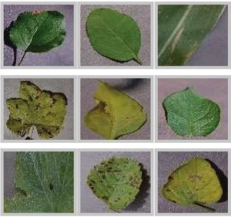
Fig. 1: Sample examples of plant leaf images.
To compare individual sample of plant leaf images taken from dataset are feed to deep learning models. The process includes classification, feature selection, feature extraction, and preprocessing. Because inaccurate data in a dataset might alter the appearance of a test, the information series technique is essential in real-time operations. As a result, it is essential to follow the unusual norm and standard while gathering statistics. Subsets of the datasets are created using an 80:20 training-to-testing ratio. While the last twenty-seven demonstrate unique plant leaf diseases, thirteen of the forty trainings that comprise our information are the healthful classes.
The data have 256×256-pixel RGB images showing results of leaves. Based on their image classifications, care was taken during the photo shoot to ensure that each image captured a single centered leaf. Additionally, the environment for shooting photos and the lighting are consistent. It is significantly more beneficial to ask questions about how to use the knowledge effectively after analyzing a variety of data.[14] Fig. 2 shows block diagram of plant leaves disease detection mechanism.
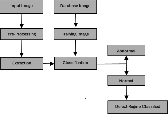
Fig. 2: Block diagram of plant leaves disease detection mechanism.
4. Pre-processing and augmentation
It is generally known that different types of factors, such as human error and noise, can be the facts obtained from any source. The set of rules can produce misleading results if it uses such data immediately. Pre-proclamation of the facts supplied is therefore a latter step. Pre-processing techniques include scaling, color space modification, picture enhancement, and noise reduction to improve the quality of the data and eliminate or minimize noise from the original input data. The act of hybrid model is evaluated in this study by enlarging the leaf picture to 224 × 224 x 3.[14] Additionally, it is significantly more beneficial to ask questions about how to use the knowledge. Fig. 3 shows the outcomes of preprocessing of the RGB images (plant leaves) using gray scale transformation. Records augmentation, which includes flips, zoom, vertical shift, and horizontal shift, is essential for training information since it increases the number of photos and reduces overfitting.
This is used encoder-decoder architecture and highly defined neural networks to apply semantic leaf disease division to a collection of plant pictures. Three distinct semantic segmentation models like Lonate-34, Pyramid Scene Parsing Network (PSPNet), and Seagate[15] were employed to detect wounds to provide a high density. After the lesions are detected, they are classified using several classifiers.
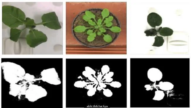
Fig. 3: Grayscale conversion of input dataset.
The plant blades are the input for both semantic segmentation techniques. PSPNet,[16] Seagate,[17] and Longett-34,[18] are two semantic segmentation models, are used to recreate model. To utilize global reference information, this modular semantic partition paradigm uses reference aggregation based on many domains. Local and global cues work together to strengthen the final restriction. Moreover, the U-Net architecture is extensively recognized for its effectiveness in the responsibilities of semantic division, creating the foundation of this technique. It can divide a wide range of gadgets, which include clinical imaging for PC pictures and prescribed in satellite TV. By combining decoder and encoder approaches, the Llenge-34 design aims to enhance partition model training and increase productivity and efficiency. It consists of a down-sampling server which shrinks input photos to exclude top level information generate predictions at the pixel level. Linknet-34 connects the coder and decoder via a jump connection. In addition, low-level features may be communicated without delay into decoders and integrated with high-degree statistics via the use of jump connections, akin to U-Net. Division is contemplated inside the object. When it comes to segmental segmentation problems, the PSP Net plays properly. By assigning a semantic label to a given image, each pixel attempts to share the semantic segmentation of the image into regions corresponding to different types of objects. Pyramid basin modules are used by the PSPN to acquire multi-paan reference facts from wonderful components of the doorway picture.[19] This makes it easier for the model to assume more pixels than are necessary, particularly for objects of different sizes. To collect contextual records, PSP Net repeatedly down samples the input characteristic map using a pyramid shape and uses global pooling at various scales. As an alternative, the conventional layers are used for characteristic combining and up sampling. Examples of jobs where PSPNET performs well and where pixel-level segmentation is required are Sean Parsing, Image Segmentation, and Pleasant-Green Object recognition. With a total of 26 convolutional layers, Seg-Net is an encoder-decoder version. The VGG16 community's development and contraction routes have thirteen Convo layers. The encoder and decoder networks are separated by two fully connected (FC) layers. The Rectified Linear Unit (ReLU) is the system that is used to easily and quickly construct function mappings.
A max-pooling operation with a stride of two comes after each layer for the down sampling of the feature map. Down sampling increases the number of channels and filter banks, typically doubling them at each step. Each encoder layer has a corresponding decoder layer, where the decoder samples the data by a factor of two before passing it to the next feature map. The primary encoder handiest has a multichannel characteristic map, but the decoder has just three channels. After map output, a multi-dimensional feature is employed to solve a 2-class problem by using the Sign ID Ed capability to separate plant pixels from the background.[20]
4.1 Image acquisition
The input information first is captured the use of a Xiaomi USB 2.0 HD webcam that supports taking pictures video datasets up to 720p and a body fee of 30 frames per 2d (fps). This enters records then undergo photograph pre-processing where the statistics are normalized into a scale of [0,1] because it consisted of pixels starting from 0-255. Upon normalization, the performance of the CNN model improves ensuring better numerical balance and quicker convergence. The input records also undergo grayscale conversion as weed detection is predicated greater upon shapes and textures than color.[11] The machine is made greater efficient by way of resizing the facts to 64×64 pixels for that reason reducing the photograph size and reducing the computational fee.[21]
4.2 Feature extraction
Now functions are being extracted from the pre-processed photo using 2D Convolution that extracts out all critical features and styles like edges and so forth.[16] It applies 32 filters of the dimensions (3×3 i.e., 64×64 in grayscale) at the input image. The 2d convolutional layer once more applies to 64 filters of the equal size. Rectified Linear Unit (ReLU) right here acts because the activation function which converts the terrible values to zero therefore introducing non-linearity. Fig. 4 shows demonstration of the Rectified Linear Unit (ReLU).
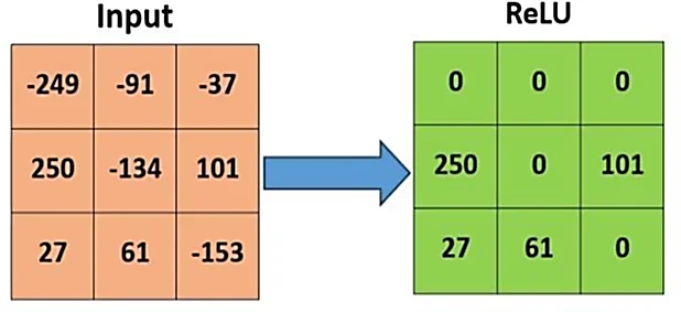
Fig. 4: A demonstration of the Rectified Linear Unit (ReLU).
The non-linearity added through the ReLU activation feature lets in the CNN network to learn extra complex patterns and functions which are beyond the linear relationships. This makes the network computationally extra green as fewer neurons prompt immediately, enhancing generalization, appearing as simple threshold capability. Compared to other activation functions such as sigmoid and tanh, it avoids costly exponential calculations, thereby enabling faster convergence during network training and helping gradients remain large during backpropagation. Fig. 5 illustrates how negative inputs are converted to zeros, introducing sparsity in the activations.[22]
5. Proposed methodology
We begin by outline the dataset, emphasizing the splitting processes, and discussing the methods of training models. Also, the suggested model's records flow diagram is displayed in Fig. 5.[23]

Fig. 5: Flow diagram of plant leaf disease classification mechanism.
5.1 Dataset description
The proposed experiment applied the Garden Village Dataset present in Kaggle which includes 20,639 photos of high decision of 38 exceptional healthful and diseased leaves bearing on 18 different species of plants, as shown in Table 2. The model implementation considers segmented images of four plants along with their diseases.
Table 2: Data specifications.
| Plant | Disease Name | Count |
|---|---|---|
| Corn | Gray leaf spot | 443 |
| Maze rust | 2193 | |
| Fit (Healthy) | 1162 | |
| Apple | Bacterial black rot | 621 |
| Healthy | 1645 | |
| Apple Scab | 630 | |
| Tomato | Septoria | 1771 |
| Early blight | 1000 | |
| Leaf mold | 952 | |
| Healthy | 1591 | |
| Grapes | Esca | 1383 |
| Siriasis | 1076 | |
| Black rot | 1180 | |
| Healthy | 423 |
5.2 Image segmentation
One crucial aspect of image processing is image division. There are several techniques for dividing pictures, including the Otsu method, K-peins clustering, borders and spot detection algorithms, etc. One of the best edge detectors is the Edge Detection as it offers the best, most dependable, and least error-prone real age point detection.
The following procedures are used to identify edges with the clever edge detector:
- Smoothing: order to smooth the photo and minimize noise, Gaussian clear out is used.
- Finding depth gradients: Wherever the picture's gradients have significant magnitudes, the edges are indicated. Large-magnitude photos' gradients are emphasized as edges.
- Non-maximum suppression: This technique eliminates erroneous reactions to component detection.
- Double Threshold: This is a criterion used to determine true edges and abilities.
- Edge tracking: The weak edges attached to the strong edge are the original or the actual edge, while the weak edges that are not attached to the strong edge are pressed.
6. Classification
6.1 Support Vector Machine (SVM) algorithm
Plant diseases are identified using the Support Vector Machines (SVM)[24] set of rules. Finding the Most Marginal Hyperplane (MMH) that divides the educational records into instructions is the aim of supervised mastering and vector space-based machine learning techniques like SVMs. This method facilitates the examination of statistics for regression analysis, classification, and grouping. The following are the steps to determine the biggest marginal hyperplane:
- Flat are recursively generated to segregate the training in the exceptional manner.
- The following step is to select for proper outcomes the hyperplane with the highest segregation from each nearby statistics component.
6.2 Convolutional Neural Networks (CNN)
Convolutional Neural Networks (CNNs) are a class of Artificial Neural Network (ANN) designed to automatically and adaptively learn the features at different levels of detail from the input data (generally images). Image processing and recognition are two main applications of CNN. They are carried out by means of an optimizer and activation capabilities.[25]
DenseNet: One shape of CNN that employs dense connections between layers is referred to as a Dense Net. These layers are linked to each other through Dense Blocks. If there are similar plant picture variants, this technique is appropriate. Apple and tomato leaves, as an instance.[26]
Efficient Net: A specific predetermined set of scaling coefficients is used by the CNN structure Efficient Net to evenly scale each dimension using the compound coefficient approach. It attains greater precision and efficiency.
Activation functions: The activation function in neural networks overseas transforming the weighted sum of inputs from nodes in a community layer into an output. ReLU (Rectified Linear Unit) is used in this model because the hidden layer's activation characteristic outputs the input instantly if it is of good quality; else, it would output 0.
f(x) = max (0, x)
The SoftMax function, which calculates the likelihood of data pertaining to the magnificence used for the multiclass concerns and returns values between 0 and, is utilized in the concluding layer:
Optimizers: Optimizers are techniques for changing a model's parameters, such as weights and study rate, to reduce losses. Adam Optimizer is one of the optimizers utilized in this version. This set of rules accelerates the gradient descent process by considering the exponentially weighted common of the gradients.[27]
Optimizers are techniques used to adjust the parameters, including weights and learning rates, of a model to minimize loss. One of the optimizers employed in this model is the Adam Optimizer, which accelerates the gradient descent process by computing an exponentially weighted average of past gradients.
Pyramid Scene Parsing Network (PSPNet) performs exceptionally well in challenging semantic segmentation scenarios. Fig. 6 shows object segmentation using semantic segmentation of the image. Additionally, the semantic segmentation input seeks to distinguish images by assigning a semantic label to each pixel. Pyramid pooling modules are used by PSPNet to extract various scale data from various regions of the original picture. This enhances the pixel forecasting capability, particularly for objects with varying sizes. PSPNet frequently down samples the input feature map and applies global pooling at multiple scales to capture contextual information. Pixel-level predictions are then generated by up sampling and combining this information. While PSPNet uses global pooling across several pyramid levels to gather context, it does not include the fusion step that is present in Feature Pyramid Network (FPN). Function combining and up-sampling are replaced with convolutional layers.[15]
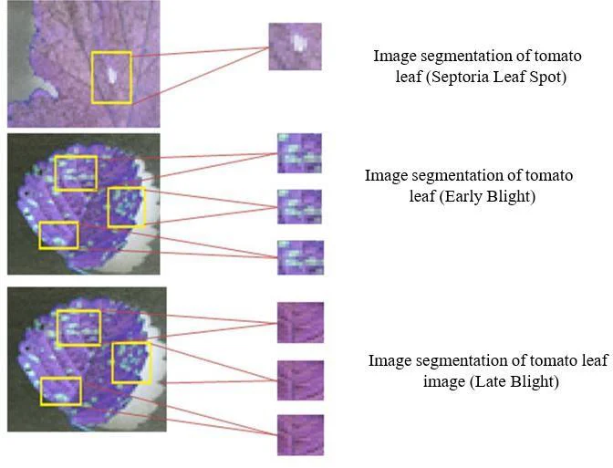
Fig. 6: Object segmentation using semantic segmentation of the image.
6.3 Convolution operation
All the layers of the CNN Network Densnet121[28] include feed-forward coupling. Each feature map from the earlier layers serves as the layer's input. The N-layer network is regarded as an example. Additionally, the feature map is then forwarded to the Nth layers' subsequent N input. Consequently, the network's dense connection is represented as an input by Equation (1) Layer.
Li = L0, L1, L2 ... LL-1 (1)
in which Li=TrL0,L1,L2,LL-1 and Li is the layer's input. Feature maps from 0 to L-1 and together make up the layers. “Density block (DB)” and “infection blocks (TB)” are the two main types of building networks. Each of the “dense layers (DL)” that make up the dense blocks consists of a layer that is 1x 1 conv and a layer that is 3 x 3 conv.
CNN architecture is known as an aggregated residual transform network, or briefly considered, the ideas of Inception Networks and Residual Networks (DenseNet). It provides the imagination of change and combines, highlighting the notion that cardinality may enhance impact. Dense Net employs a split, re-creation, and merging block that incorporates several ameliorations. As a result of these modifications, a huge number of representations and a broad spectrum of abstractions were captured. The transition blocks' 1 x 1 CNN layers and 2 x 2 Pooling layers are situated dense blocks. The layers of batch normalization are arranged in descending order. DenseNet121 is a variant of the Dense Net architecture, which utilizes convolution operations applied to feature maps with real-valued inputs.[29] Fig. 7 shows 2D convolution level function of a CNN. These layers in each DenseNet121 are illustrated in Figs. 7 and 8. Convolution is an operation that uses real numbers as parameters and is applied to two features. The convolution process involved a multidimensional vector (tensor). The kernel, which is adjusted during training, is essentially a multidimensional parameter tensor. For instance, a two-dimensional kernel represented by K is frequently employed when image I is used as input.
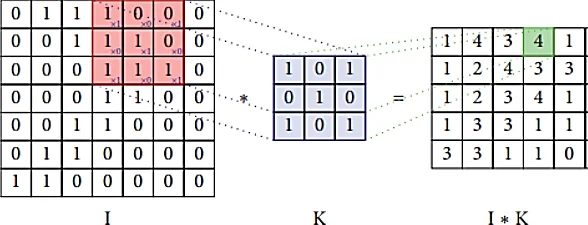
Fig. 7: 2D Convolution level function of a CNN.
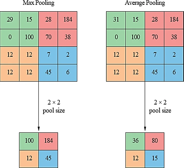
Fig. 8: Maximum clustering of left and middle-right pooling in a pooling function.
- Pooling: A CNN typically consists of three main layers. The functioning of the entry facts is folded at the community level. This phase is sometimes referred to as the thought level.[30] The last stage is the be-part feature, which substitutes a statistical precis produced by the previous neural network layer position for the prior output or network output. The implementation of the 2×2 pooling method is depicted in Fig. 8. There are two types of pooling: Maximum Pooling and Average Pooling. Max pooling selects the highest value in each region as illustrated in Fig. 8, by the 2×2 Pooling method. This reduces the data size by a factor of 4. Average pooling, on the other hand, computes the arithmetic meaning of the values in the region.[31]
- Model and Architectures: The model was chosen to address the specific problem, taking into account the many possible designs available and the widespread use of convolutional neural networks in various modern computer vision and predictive tasks.[16] It is also important to consider the trade-off between the number of layers and parameters to train (and the computational expenses that are required for training), especially the ones that have been well established in the literature and have shown state-of-the-art performance in computer vision applications. In this regard, we chose to use convolutional neural networks with fewer parameters than both popular solutions in the literature, such as the standard for our tasks. The resulting architectures used are therefore:
- LeNet: Designed for the purpose of handwritten digit recognition, this network has two layers of convolution which are pooled using max pooling to get features. Finally, to the outlet category, we apply a final convolutional layer using dense layers.[17]
- AlexNet: This Network consists of five preliminary convolutional layers. screen 3 layers which only two layers Z-layers is not fully attached within the quit to provide the classification. It aims to use convolutional, neural network architecture with right overall performance mentioned in the corresponding studies.
- MobileNet: This convolutional neural network is designed on deep separable convolution operations, which reduces the burden of workload to execute the internal operations the initial layers of this mobile-targeted devices and embedded devices.[28]
- ShuffieNet: It is primarily built upon two operations, which the authors defined: the so-called the group convolutions that could be foreroi4ing, and may be multiple convolutions on part of the input channels, and the channel shuffie, which uses a random blend the output channels of the convolutions inside the organization. This structure, advocates say supports a reasonable accuracy with a low computing cost.[32]
- EffNet: Along the lines of utilizing in-depth separable convolution, which is akin to MobileNet design.[32] and ShuffieNet networks; however, it presents a new convolution block that reduces the computational cost and outperforms state-of-the-art for certain known databases.[33]
- Sheaf Attention Network: Efficient segmentation and classification using Convolutional neural networks with Sheaf Attention Networks (CSAN).[34]
7. Results and discussion
It should be noted that the total number of parameters is smaller than that of the VGG16 and VGG19 designs,[35] indicating that, under the circumstances examined, we may find that their combination may end up being less expensive than well-known architectures in the literature. The architecture under consideration was trained using the previously described methods, and their individual performance in the test set was assessed.
In supervised learning, a collection of instances (input and intended output) is presented to train the classifier. In supervised methods, the model is trained to produce the desired output but from a training set. This training data set consists of correct and incorrect outputs so that the model can evolve. According to this information, it is expected that the classifier should operate in a linear or non-linear fashion and accurately predict the output for newly input data. Considering the SVM, they use an ideal separation hyperplane that is precisely in the middle of the two classes margins to partition the feature. Nonlinear Radial Basis Function (RBF), quadratic, polynomial, Gaussian and two-layer perceptions are non-linear functions used in the SVM analysis. This process is for improving the separation margin. After that, an SVM classifier is used to analyses the images to identify the plant. The illness classifier and severity classifier modules employ deep learning techniques to improve performance and get more precise findings.
7.1 Using deep learning (Image-based approach)
The recent most popular and efficient algorithm is Convolutional Neural Network (CNN). It will be trained to categorize leaf images into groups that are healthy or ill.
Technologies & Tools:
- Python 3.13.3
- TensorFlow/Keras/PyTorch
- OpenCV (for preprocessing)
- Pre-trained Models like MobileNet, ResNet for transfer learning
Workflow:
- Dataset: Plant Village Dataset.
- Preprocess Images: Resize, Normalize, Augment.
- Classification: CNN Model (a pre-trained model).
- Evaluation metrics: Accuracy, Confusion Matrix, F1-score.
7.2 Evaluation metrics
The outcome of plant leaf lesion detection is tested with various evaluation criteria, such as precision, recall, F1-score, accuracy, Jaccard, and dice coefficient. The precision (Pre) in Equation (2) is the ratio of the correctly detected targets to all the targets detected by the proposed model.[34]
Pre = TP / (TP + FP) (2)
where,
TP = True Positive
TN = True Negative
FP = False Positive
FN = False Negative
Recall, often called 'Rec' is the percentage of targets that the model got right. You can find the recall rate using the formula in Equation (3). 'FN' means that the model didn't correctly identify the target, which in this case is leaf lesions.
Rec = TP / (TP + FN) (3)
The F1 score is another way to measure how well a classification model is doing, taking both memory and precision into account. It gives a good picture of both Precision and Recall since it combines them into one score. It is greatest when Precision and Recall are identical, according to Equation (4).
F1 Score = (2 × Pre × Rec) / (Pre × Rec) (4)
Accuracy is one metric used to evaluate classification methods. Accuracy may be defined as the proportion of accurate predictions our model produced. Accuracy is defined formally as the ratio of correctly labelled pictures to all sample. Accuracy is represented mathematically in Equation (5).
Accuracy = (TP + TN) / (TP + FP + FN + TN) (5)
The intersection of spatial overlap is measured using the union size of two label sets, based on the Jaccard Index (JAC) in Equation (6).
JAC = TPosi / (TPosi + TPosi + Fneg) (6)
The Dice Similarity Coefficient (DSC) shows how similar two binary images are, with zero meaning no overlap and one meaning complete overlap. We get the segmentation result and DSC values from a specific Equation (7).
DCS = 2TPosi / (2TPosi + TPosi + Fneg) (7)
The model classifies many images by predicting how likely it is that each image falls into a particular class.
7.3 Experimental analysis
7.3.1 Metric value
The proposed prototype in this study is trained and developed using a standard self-developed dataset. The prototype was being implemented using CNN as well as YOLOv4 deep learning algorithms and after successful testing phase, the results have been concluded and compiled evaluation metrics.
The results of each technique have been thoroughly evaluated ensuring untampered standards and accurate real-world simulation. Table 3 summarizes the result metrics of YOLOv4 technique that was implemented on the very same setup for a through comparison. Fig. 9 shows results using YOLOv4 technique.
Table 3: Results during field testing using YOLOv4.
| Field trial | True cases | False cases | % Error | % Success | ||
|---|---|---|---|---|---|---|
| TN | TP | FN | FP | |||
| 1 | 6 | 11 | 2 | 1 | 15 | 85 |
| 2 | 6 | 12 | 2 | 0 | 10 | 90 |
| 3 | 6 | 12 | 0 | 2 | 10 | 90 |
| 4 | 3 | 16 | 0 | 1 | 5 | 95 |
| 5 | 7 | 12 | 1 | 0 | 5 | 95 |
| 6 | 11 | 9 | 0 | 0 | 0 | 100 |
| 7 | 8 | 12 | 0 | 0 | 0 | 100 |
| 8 | 4 | 16 | 0 | 0 | 0 | 100 |
| 9 | 14 | 6 | 0 | 0 | 0 | 100 |
| 10 | 10 | 10 | 0 | 0 | 0 | 100 |
| Total | 75 | 116 | 5 | 4 | - | - |
| Average | - | - | - | - | 4.5 | 95.5 |
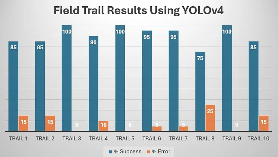
Fig. 9: Results of field trail using YOLOv4.
Using Equation (5) we can calculate the value of accuracy as follows:
Accuracy = (103 + 79) / (103 + 79 + 6 + 12) = 91.0%
Similarly, using Equation (2) and (3) the precision and recall calculated:
Precision = 103 / (103 + 6) = 94.49%
Recall = 103 / (103 + 12) = 89.56%
Now, Equation (4) is being used to calculate the F1 Score for technique:
F1 Score = (2 × 0.9449 × 0.8956) / (0.9449 × 0.8956) = 91.96%
Table 4 summarizes the result metrics of CNN technique that was implemented on the very same setup for a through comparison. Fig. 10 shows results using CNN technique.
Accuracy = (116 + 75) / (116 + 75 + 4 + 5) = 91.50%
Similarly, using Equation (2) and (3) the precision and recall calculated:
Precision = 116 / (116 + 4) = 96.66%
Recall = 116 / (116 + 5) = 95.86%
Now, Equation (4) is being used to calculate the F1 Score for technique:
F1 Score = (2 × 0.9666 × 0.9586) / (0.9666 × 0.9586) = 96.25%
From the above equations, it can be clearly observed that the CNN technique has completely outperformed the YOLOv4 algorithm and proven its proficiency in accurate object detection and recognition. This study was to determine the optimal performance of various deep learning (DL) algorithms in classification and precise elimination of weeds amongst the crop field.
Table 4: Results during field testing using CNN.
| Field Trial | True Cases | False Cases | % Error | % Success | ||
|---|---|---|---|---|---|---|
| TN | TP | FN | FP | |||
| 1 | 6 | 11 | 2 | 1 | 15 | 85 |
| 2 | 6 | 12 | 2 | 0 | 10 | 90 |
| 3 | 6 | 12 | 0 | 2 | 10 | 90 |
| 4 | 3 | 16 | 0 | 1 | 5 | 95 |
| 5 | 7 | 12 | 1 | 0 | 5 | 95 |
| 6 | 11 | 9 | 0 | 0 | 0 | 100 |
| 7 | 8 | 12 | 0 | 0 | 0 | 100 |
| 8 | 4 | 16 | 0 | 0 | 0 | 100 |
| 9 | 14 | 6 | 0 | 0 | 0 | 100 |
| 10 | 10 | 10 | 0 | 0 | 0 | 100 |
| Total | 75 | 116 | 5 | 4 | - | - |
| Average | - | - | - | - | 4.5 | 95.5 |
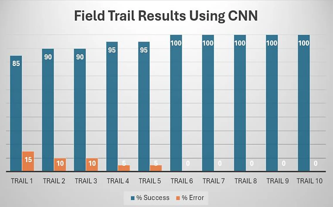
Fig. 10: Results of field trail using CNN.
CNN classification and YOLOv4 supervised algorithms for a comparison-based study and detailed analysis in the search for the best algorithm to be implemented.
Fig. 11 shows the Confusion Matrix for YOLOv4 technique. YOLOv4 in field testing lacks true positive cases (TP = 103), whereas its greater true negative (TN = 79) and false negative (FN = 12).
Fig. 12 shows confusion matrix for CNN technique. It could be truly determined that the CNN method has absolutely outperformed the YOLOv4 algorithm and confirmed its scalability in correct object detection and recognition. The YOLOv4 in field testing lacks true positive cases (TP = 103), whereas its greater true negative (TN = 79) and false negative (FN = 12) values result in lower precision as compared to CNN.[22]
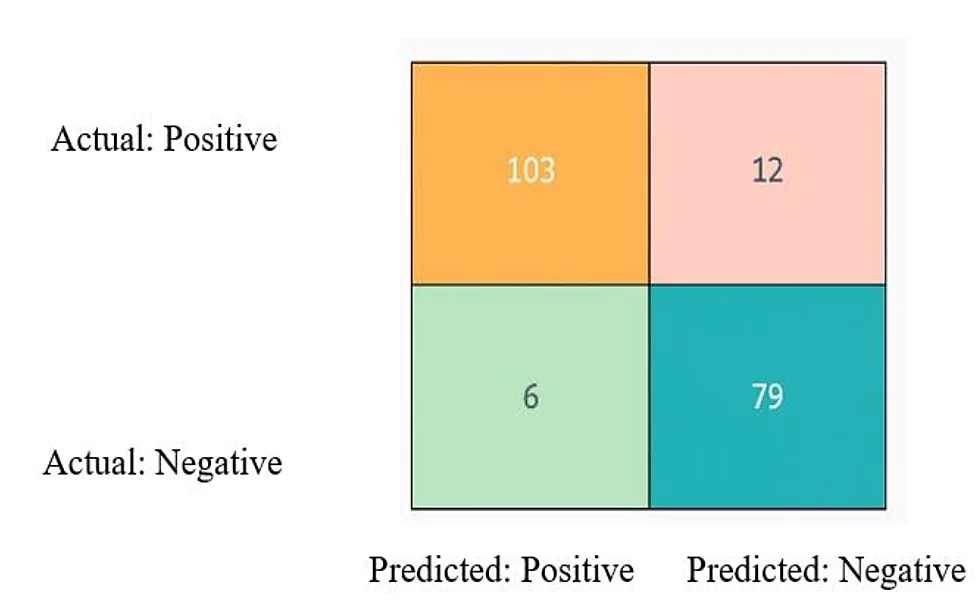
Fig. 11: Confusion matrix for YOLOv4 technique.
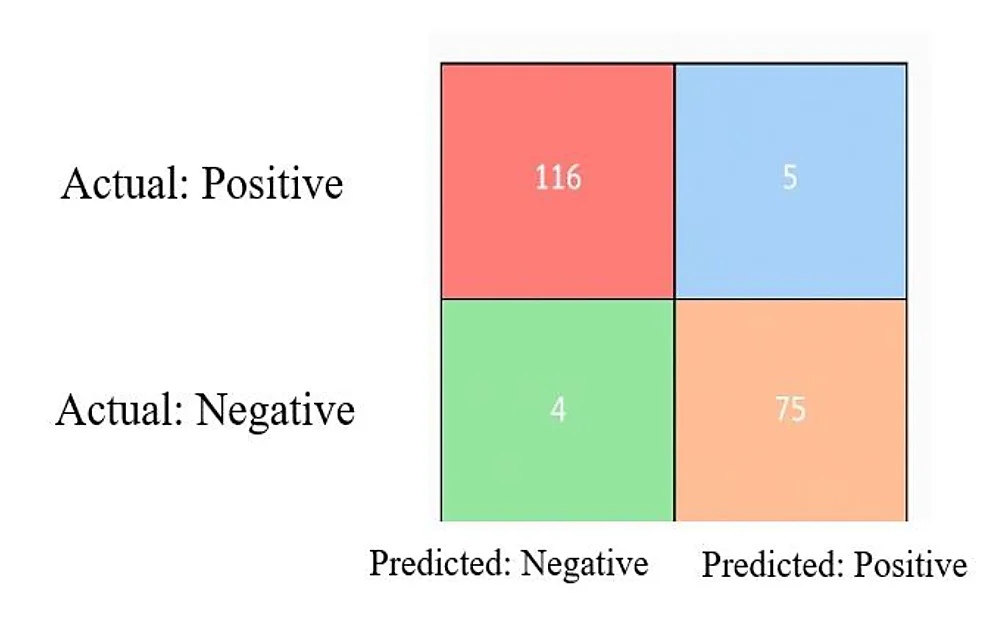
Fig. 12: Confusion matrix for CNN technique.
Traditional ML + Image Features:
- Use models like SVM, Random Forest, KNN for classification.
- Extract features like color histograms, shape descriptors, texture.
Web App Integration:
Once we have a model, we have:
- Deploy via Flask backend.
The homepage layout of this graphical user interface is displayed in Fig. 13, while the functional user interface of the proposed prediction model is shown in Fig. 14.
We looked at different plant disease datasets from Kaggle, including apples, corn, tomato, and grapes. The test scores for the disease and severity classifiers are shown in Table 5.
This study was to determine the optimal performance of various deep learning (DL) algorithms in classification of plant leaf diseases. CNN classification and YOLOv4 supervised algorithms for a comparison-based study and detailed analysis in the search for the best algorithm to be implemented.
Table 5: Test scores for classifying plant diseases.
| Plant | Disease name | Accuracy (%) |
|---|---|---|
| Apple | Healthy | 92.5 |
| Apple scab | 100 | |
| Black rot | 100 | |
| Corn | Healthy | 100 |
| Common rust | 100 | |
| Gray leaf spot | 57.5 | |
| Grapes | Healthy | 90 |
| Black rot (High) | 100 | |
| Black rot (Low) | 85 | |
| Esca (High) | 90 | |
| Esca (Low) | 100 | |
| Siriasis (High) | 95 | |
| Siriasis (Low) | 100 | |
| Tomato | Healthy | 100 |
| Leaf mold | 100 | |
| Septoria | 100 | |
| Early blight | 95 |
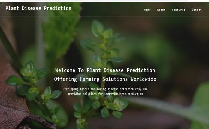
Fig. 13: Homepage of graphical user interface.
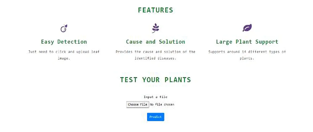
Fig. 14: User interface of proposed prediction model.
7.4 Discussion
Deep learning (DL) is changing the scenario when it comes to diagnosing plant diseases using digital images. To get the right response quickly, the models need to be fast and accurate. The design of the network chosen will depend on to improve or reduce accuracy of prediction model. If we need to change things up often, Dense Net (CNN) is the quickest option, though it can be a bit unstable. On the other hand, if we want top-notch accuracy, we might want to look at GoogLeNet or AlexNet. They found that while InceptionV3 had the lowest accuracy in their tests, AlexNet, though not performing as well as expected, still outperformed it overall.
The prototype in this study is being developed and implemented using CNN classification and YOLOv4 supervised learning algorithms for a comparison-based study and detailed analysis in the search for the best algorithm to be implemented. This step is particularly necessary for accurate classification of plant leaf diseases detection on different geographical locations and regions. Fig. 15 shows the accuracy comparison by various detection techniques. Fig. 16 shows the results of comparision between YOLOv4 vs CNN.
Now as we observe in Table 6, a comparison has been stated amongst accuracies of four other methods being generally used in effective object detection and classifications with the two root methods mentioned in this study. Jun Zhang et al.[33] mentioned in his study about the higher accuracy of the original ViT model due to its stronger sequence modelling abilities and unique capabilities to capture long-range dependencies. But when we carefully consider both CNN, ViT and YOLOv4 in a comprehensive way, then the CNN model due to its better balance for local and global features, results in an overall better performance and improved classification.
Additionally, despite having several depth layers, the deepest networks are ResNet50, ResNet101, and InceptionV3 are showed comparatively low accuracy. Lastly, a time and performance analysis of several CNNs was suggested.
Table 6: Comparison with other detection techniques.
| Model Name | Accuracy (%) |
|---|---|
| VGG16 | 86.21 |
| GoogleNet | 79.23 |
| AlexNet | 80.09 |
| ViT | 89.09 |
| YOLOv4 | 91.00% |
| CNN | 95.50% |
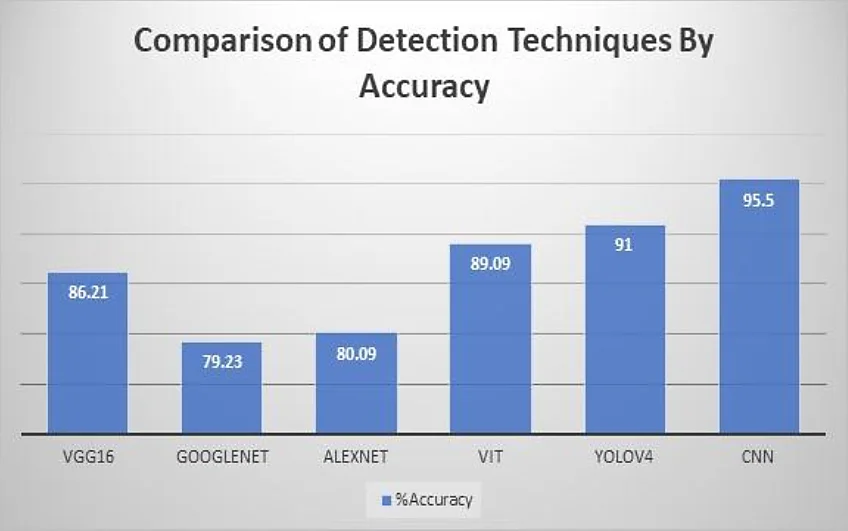
Fig. 15: Accuracy comparison by various detection techniques (deep learning algorithms).
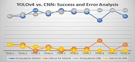
Fig. 16: Results of YOLOv4 vs CNN.
8. Conclusion and future scope
The main goal of the plant disease detection and severity classification model is to uses images of leaves of infected plant species to precisely identify plant diseases and their severity levels. This model focuses on using advanced image processing techniques based on CNN to determine multi-class detection of plant leaf disease detection, which helps to extract important characteristics required for efficient categorization. Utilizing these extracted metrics, the model facilitates early and accurate disease identification in a variety of plants, allowing producers to take prompt and suitable corrective action. Apple, corn, grapes, and tomatoes are the four plant species on which the system has been extensively tested; each of these plant species has two to three different diseases. This makes the model approachable and useful for actual agricultural applications by enabling effective and straightforward forecasts. Both YOLOv4 and CNN-based models exhibit notable gains in plant disease detection accuracy, according to the experimental investigation. The addition of severity categorization improves the model's usefulness in practice by revealing information about the disease's course in addition to its identification.
Funding Declaration
Data Availability Statement
Conflict of Interest
Artificial Intelligence (AI) Use Disclosure
Supporting Information
References
- [1] K. Kc, Z. Yin, D. Li, Z. Wu, Impacts of background removal on convolutional neural networks for plant disease classification in-situ, Agriculture, 2021, 11, 827, doi: 10.3390/agriculture11090827.
- [2] Y. Gai, H. Wang, Plant disease: a growing threat to global food security, Agronomy, 2024, 14, 1615, doi: 10.3390/agronomy14081615.
- [3] M. Bhagat, D. Kumar, I. Haque, H.S. Munda, R. Bhagat, Plant leaf disease classification using grid search based SVM, In 2nd International conference on data, engineering and applications (IDEA), IEEE, 2020, 1–6.
- [4] V. S. Dhaka, S. V. Meena, G. Rani, D. Sinwar, M. F. Ijaz, M. Woźniak, A survey of deep convolutional neural networks applied for prediction of plant leaf diseases, Sensors, 2021, 21, 4749, doi: 10.3390/s21144749.
- [5] V. P. Ananthi, Fused segmentation algorithm for the detection of nutrient deficiency in crops using SAR images, In Artificial Intelligence Techniques for Satellite Image Analysis, Cham: Springer International Publishing, 2019, 137-159.
- [6] M. H. Saleem, J. Potgieter, K. M. Arif, Plant disease classification: a comparative evaluation of convolutional neural networks and deep learning optimizers, Plants, 2020, 9, 1319, doi: 10.3390/plants9101319.
- [7] K. Zou, H. Wang, T. Yuan, C. Zhang, Multi-species weed density assessment based on semantic segmentation neural network, Precision Agriculture, 2023, 24, 458-481, doi: 10.1007/s11119-022-09953-9.
- [8] Y. Majeed, J. Zhang, X. Zhang, L. Fu, M. Karkee, Q. Zhang, M. D. Whiting, Deep learning-based segmentation for automated training of apple trees on trellis wires, Computers and Electronics in Agriculture, 2020, 170, 105277, doi: 10.1016/j.compag.2020.105277.
- [9] R. Rinu, S. H. Manjula, Plant disease detection and classification using CNN, International Journal of Recent Technology and Engineering, 2021, 10, doi: 10.35940/ijrte.C6458.0910321.
- [10] S. M. Hassan, A. K. Maji, Plant disease identification using a novel convolutional neural network, IEEE Access, 2022, 10, 5390-5401, doi: 10.1109/ACCESS.2022.3141371.
- [11] P. Kaur, S. Harnal, V. Gautam, M. P. Singh, S. P. Singh, A novel transfer deep learning method for detection and classification of plant leaf disease, Journal of Ambient Intelligence and Humanized Computing, 2023, 14, 12407-12424, doi: 10.1007/s12652-022-04331-9.
- [12] S. S. Harakannanavara, J. M. Rudagi, V. I. Puranikmath, A. Siddiqua, R. Pramodhini, Plant leaf disease detection using computer vision and machine learning algorithms, Global Transitions Proceedings, 2022, 3, 305–310, doi: 10.1016/j.gltp.2022.03.016.
- [13] M. Aggarwal, V. Khullar, N. Goyal, A. Singh, A. Tolba, E. B. Thompson, S. Kumar, Pre-trained deep neural network-based features selection supported machine learning for rice leaf disease classification, Agriculture, 2023, 13, 936, doi: 10.3390/agriculture13050936.
- [14] R. Sharma, V. Kukreja, Amalgamated convolutional long term network (CLTN) model for lemon citrus canker disease multi-classification, In 2022 International conference on decision aid sciences and applications (DASA), IEEE, 326-329.
- [15] A. Chug, A. Bhatia, A. P. Singh, D. Singh, A novel framework for image-based plant disease detection using hybrid deep learning approach, Soft Computing, 2023, 27, 13613-13638, doi: 10.1007/s00500-022-07177-7.
- [16] A. Sulaiman, V. Anand, S. Gupta, M. S. Al Reshan, H. Alshahrani, A. Shaikh, M. A. Elmagzoub, An intelligent LinkNet-34 model with EfficientNetB7 encoder for semantic segmentation of brain tumor, Scientific Reports, 2024, 14, 1345, doi: 10.1038/s41598-024-51472-2.
- [17] M. Chhabra, R. Kumar, A smart healthcare system based on classifier DenseNet 121 model to detect multiple diseases, In Mobile radio communications and 5G networks: proceedings of second MRCN 2021, Singapore: Springer Nature Singapore, 2022, 297-312.
- [18] I. Ahmad, M. Hamid, S. Yousaf, S. T. Shah, M. O. Ahmad, Optimizing pretrained convolutional neural networks for tomato leaf disease detection, Complexity, 2020, 2020, 8812019, doi: 10.1155/2020/8812019.
- [19] T. Y. Lin, P. Dollár, R. Girshick, K. He, B. Hariharan, S. Belongie, Feature Pyramid Networks for Object Detection, In Proceedings of the IEEE conference on computer vision and pattern recognition, IEEE, 2017, 2117-2125, doi: 10.1109/CVPR.2017.106.
- [20] Y. M. Abd Algani, O. J. Marquez Caro, L. M. Robladillo Bravo, C. Kaur, M. Saleh Al Ansari, B. Kiran Bala, Leaf disease identification and classification using optimized deep learning, Measurement: Sensors, 2023, 25, 100643, doi: 10.1016/j.measen.2022.100643.
- [21] A. Pal, V. Kumar, AgriDet: Plant leaf disease severity classification using agriculture detection framework, Engineering Applications of Artificial Intelligence, 2023, 119, 105754, doi: 10.1016/j.engappai.2022.105754.
- [22] V. Sharma, A. K. Tripathi, H. Mittal, DLMC-Net: Deeper light weight multi-class classification model for plant leaf disease detection, Ecological Informatics, 2023, 75, 102025, doi: 10.1016/j.ecoinf.2023.102025.
- [23] S. R. G. Reddy, G. P. S. Varma, R. L. Davuluri, Resnet-based modified reddeer optimization with DLCNN classifier for plant disease identification and classification, Computers and Electrical Engineering, 2023, 105, 108492, doi: 10.1016/j.compeleceng.2022.108492.
- [24] S. S. Salve, S. P. Narote, Iris recognition using SVM and ANN, In 2016 International Conference on Wireless Communications, Signal Processing and Networking (WiSPNET), IEEE, 2016, 474-478, doi: 10.1109/WiSPNET.2016.7566179.
- [25] A. Arshaghi, M. Ashourian, L. Ghabeli, Potato diseases detection and classification using deep learning methods, Multimedia Tools and Applications, 2023, 82, 5725-5742, doi: 10.1007/s11042-022-13390-1.
- [26] S. K. Sahu, M. Pandey, An optimal hybrid multiclass SVM for plant leaf disease detection using spatial Fuzzy C-Means model, Expert Systems with Applications, 2023, 214, doi: 10.1016/j.eswa.2022.118989.
- [27] P. Singh, P. Singh, U. Farooq, S. S. Khurana, J. K. Verma, M. Kumar, Cotton LeafNet: Cotton plant leaf disease detection using deep neural networks, Multimedia Tools Applications, 2023, 82, 37151-37176, doi: 10.1007/s11042-023-14954-5.
- [28] A. M. Mishra, Y. Shahare, V. Gautam, Analysis of weed growth in rabi crop agriculture using deep convolutional neural networks, Journal of Physics: Conference Series, 2020, 2070, 01210, doi: 10.1088/1742-6596/2070/1/012101.
- [29] D. Hughes, M. Salathé, An open access repository of images on plant health to enable the development of mobile disease diagnostics, arXiv preprint arXiv:1511.08060, 2015.
- [30] M. N. Rajesh, B. S. Chandrasekar, Prostate gland segmentation using semantic segmentation models u-net and linknet, International Journal of Engineering Trends and Technology, 2022, 70, 252-271, doi: 10.14445/22315381/IJETT-V70I12P224.
- [31] S. Dhalla, J. Maqbool, T. S. Mann, A. Gupta, A. Mittal, P. Aggarwal, K. Saluja, M. Kumar, S. S. Saini, Semantic segmentation of palpebral conjunctiva using predefined deep neural architectures for anemia detection, Procedia Computer Science, 2023, 218, 328-337, doi: 10.1016/j.procs.2023.01.015.
- [32] V. Shwetha, A. Bhagwat, V. Laxmi, LeafSpotNet: A deep learning framework for detecting leaf spot disease in jasmine plants, Artificial Intelligence in Agriculture, 2024, 12, 1-18, doi: 10.1016/j.aiia.2024.02.002.
- [33] J. Zhang, Weed recognition method based on hybrid CNN-transformer model, Frontiers in Computing and Intelligent Systems, 2023, 11, 12345-12356, doi: 10.54097/fcis.v4i2.10209.
- [34] S. S. Salve, S. P. Narote, Performance evaluation of efficient segmentation and classification-based iris recognition using sheaf attention network, Journal of Visual Communication and Image Representation, 2024, 103, 104262, doi: 10.1016/j.jvcir.2024.104262.
- [35] S. S. Salve, S. S. Chakraborty, S. Gandhewar, S. S. Girhe, A deep learning framework for smart agriculture: real time weed classification using convolutional neural network, Journal of Smart Sensors and Computing, 2025, 1, 25205, doi: 10.64189/ssc.25205.
Publisher Note: The views, statements, and data in all publications solely belong to the authors and contributors. GR Scholastic is not responsible for any injury resulting from the ideas, methods, or products mentioned. GR Scholastic remains neutral regarding jurisdictional claims in published maps and institutional affiliations.
Open Access
This article is licensed under a Creative Commons Attribution-NonCommercial 4.0 International License, which permits the non-commercial use, sharing, adaptation, distribution and reproduction in any medium or format, as long as appropriate credit to the original author(s) and the source is given by providing a link to the Creative Commons License and changes need to be indicated if there are any. The images or other third-party material in this article are included in the article's Creative Commons License, unless indicated otherwise in a credit line to the material. If material is not included in the article's Creative Commons License and your intended use is not permitted by statutory regulation or exceeds the permitted use, you will need to obtain permission directly from the copyright holder. To view a copy of this License, visit: https://creativecommons.org/licenses/by-nc/4.0/
© The Author(s) 2025